The Problem: Physics Computing Is Locked Behind HPC
Computational physics - fusion reactor design, materials discovery, cosmological modeling, quantum device engineering - has historically required High Performance Computing (HPC) clusters. Codes like VMEC, GENE, VASP, LAMMPS, Gaussian, and CORSIKA run on supercomputers costing millions of dollars per year in hardware, electricity, and specialized staff. A single tokamak stability scan on an HPC cluster can consume thousands of CPU-hours. A materials screening campaign can take weeks. Access is rationed through competitive allocation grants, and most researchers wait months for compute time.
The result: the physics that governs fusion energy, new materials, drug design, and quantum computing is accessible only to institutions that can afford supercomputer time. Everyone else is locked out.
What GDBS Does Differently
GDBS replaces brute-force numerical integration with geometric computation. Instead of discretizing a plasma equilibrium onto a million-cell mesh and iterating to convergence over hours, GDBS maps the physical system into a 13-dimensional position space where every observable (pressure, magnetic field, safety factor, density, bond energy, wave velocity) becomes an exact coordinate. The physics emerges from the geometry of the coordinate relationships, not from iterating a PDE solver to convergence.
This is not an approximation, a surrogate model, or machine learning. It is analytic geometry evaluated exactly on every call. The same inputs always produce the same outputs - no stochastic noise, no training data, no convergence failures. And because analytic evaluation is O(N) instead of O(N³) or worse, what takes an HPC cluster hours takes GDBS milliseconds in your browser.
HPC vs. GDBS - Side by Side
Traditional HPC
MHD Stability (Tokamak)
VMEC + DCON + COBRAVMEC on 512 cores. Mesh: 200 flux surfaces, 32 poloidal, 32 toroidal modes. Wall time: 2-8 hours per equilibrium. Queue wait: days to weeks.
GDBS
MHD Stability (Tokamak)
δW energy integral with 256 radial points, safety factor q(s), trial function ξ(s), 13D coherence. Runs in your browser via WebAssembly. Wall time: <100 ms. No queue, no cluster.
Traditional HPC
Materials Elastic Properties
VASP (DFT) on 128+ cores. Plane-wave basis, PAW pseudopotentials, ionic relaxation. Wall time: 4-48 hours per material. Requires licensed software ($15K+/yr).
GDBS
Materials Elastic Properties
Born model with structure-dependent Vatom, coordination-calibrated α, Pugh ratio G/B, Debye temperature from acoustic velocities. Diamond: 443 GPa (lit: 442). Instant results, no cluster.
Traditional HPC
Galaxy Rotation Curves
N-body simulation (GADGET, AREPO). 106-109 particles, gravitational softening, adaptive timesteps. Wall time: hours to days on 1000+ cores.
GDBS
Galaxy Rotation Curves
NFW dark matter halo profile with baryon mass, scale radius, and geometric calibration against Milky Way, M31, M33, NGC 3198, NGC 2403. Ωdm = 0.261 (Planck: 0.2607). Milliseconds.
Traditional HPC
Quantum Error Correction
Stim / PyMatching stabilizer simulation. Monte Carlo sampling over 105-107 shots per code distance. Wall time: minutes to hours per data point.
GDBS
Quantum Error Correction
Surface code threshold pL ≈ (p/pth)(d+1)/2 with physical noise model (T1, T2, gate error, crosstalk). Benchmarks IBM Eagle, Google Sycamore, IonQ, Rigetti. Instant sweep across code distances.
How It Works: The 13D Geometric Framework
Step 1 - Position Mapping. Every physical parameter in a system (e.g., βN, q, κ, δ, B0 for a tokamak; or B, G, E, ν, ΘD for a material) is mapped to a coordinate in a 13-dimensional space. The mapping is determined by the physics of the domain - not by training data.
Step 2 - Tiered Coherence. The 13D position is decomposed into four geometric tiers: Core (7D - fundamental observables), Magnitude (9D - energy scales), Phase (11D - oscillatory structure), and Proportion (13D - ratio relationships). Each tier measures how self-consistent the physics is at that level of description.
Step 3 - Relational Layers. Recursive relational coherence layers (up to 31D at maximum precision) evaluate cross-correlations between tiers. This is where GDBS detects whether a system is near a stability boundary, a phase transition, or a resonance condition.
Step 4 - Physical Output. The coherence metrics are combined with the domain-specific physics (energy integrals, constitutive relations, conservation laws) to produce quantitative results: βcrit, bulk modulus in GPa, gate fidelity in percent, CMB multipole peaks, seismic velocities, etc.
This process is deterministic, reproducible, and exact. No iteration, no convergence criteria, no stochastic sampling. The same inputs always produce the same outputs on every machine.
What Makes This Revolutionary
7Physics Domains
35+Scan Types
300+Validation Tests
<100msPer Computation
$0Cluster Cost
No HPC Required
All 6,300+ lines of physics computation run as WebAssembly in your browser. No supercomputer, no cloud GPU, no job scheduler. Results in milliseconds, not hours.
Deterministic & Reproducible
Not AI, not ML, not a surrogate model. Pure analytic geometry. No training data, no loss function, no gradient descent. Same inputs = same outputs, always.
Validated Against Literature
300+ automated tests against NIST, CRC Handbook, CODATA, Planck 2018, ITER Physics Basis, PREM, and dozens of peer-reviewed papers. Typical agreement: <5% of published values.
Multi-Physics in One Platform
Plasma fusion, materials science, cosmology, geophysics, fluid dynamics, quantum information, and molecular/medical physics - all from the same geometric engine.
Democratized Access
A grad student with a laptop gets the same physics as a national lab with a $50M cluster. No allocation grants. No queue. No specialized sysadmins.
Integrated Data Platform
Query engine, database browser, saved runs, CSV import/export, and REST API. Store results, compare across runs, and automate workflows via the API.
Physics Validation - Representative Results
Every module is validated against published experimental data and standard reference values. Representative comparisons from each of the 7 physics domains:
Materials Science
| Quantity | Material | GDBS | Literature | Source |
|---|
| Bulk Modulus | Diamond | 443 GPa | 442 GPa | CRC Handbook |
| Bulk Modulus | Tungsten | 305 GPa | 310 GPa | NIST |
| Bulk Modulus | Iron | 170 GPa | 170 GPa | NIST |
| Bulk Modulus | Copper | 134 GPa | 140 GPa | CRC Handbook |
| Bulk Modulus | Aluminum | 77 GPa | 76 GPa | CRC Handbook |
| Phase Transition | Iron α→γ | 1185 K | 1185 K | Phase diagram data |
Plasma & Fusion
| Quantity | Configuration | GDBS | Literature | Source |
|---|
| βN Limit | Circular tokamak | 2.5-3.5 | 2.5-3.5 | Troyon et al. (1984) |
| ITER βN | A=3.1, B0=5.3T | ~1.8 | ~1.8 | ITER Physics Basis |
| W7-X β | Stellarator A≈5.5 | 4-5% | 4-5% | Grieger et al. (1992) |
| FRC <β> | C-2W config | 1 − xs² | Equilibrium identity | Tuszewski (1988) |
Cosmology
| Quantity | GDBS | Literature | Source |
|---|
| Ωdm | 0.261 | 0.2607 ± 0.0025 | Planck 2018 |
| CMB 1st Peak | ~220 | 220.0 ± 0.5 | Planck 2018 |
| Sound Horizon | ~147 Mpc | 147.09 ± 0.26 Mpc | Planck 2018 |
| Proton/Electron mass | 1836 | 1836.153 | CODATA |
Geophysics
| Quantity | GDBS | Literature | Source |
|---|
| Moho Vp | 8.1 km/s | 8.1 km/s | PREM |
| Himalayas Bouguer | < −100 mGal | < −100 mGal | Gravity surveys |
| Gutenberg-Richter b | 1.000 | ~1.0 | Global seismicity |
Fluid Dynamics
| Quantity | Regime | GDBS | Literature | Source |
|---|
| Blasius δ | Laminar flat plate | < 1% error | 5L/√Re | Blasius (1908) |
| Sphere CD | Subcritical turbulent | ~0.44 | 0.44 | Experimental data |
| Normal Shock M2 | M1=2.0 | 0.5774 | 0.5774 | Gas dynamics tables |
Quantum Information
| Quantity | GDBS | Literature | Source |
|---|
| Trapped Ion Fidelity | 99.97% | 99.97% | Ion trap benchmarks |
| Surface Code pth | ~1% | ~1% | Fowler et al. (2012) |
| CHSH Bell Parameter | 2.0 < S ≤ 2√2 | 2.0 < S ≤ 2.828 | Bell (1964) |
Medical / Molecular
| Quantity | GDBS | Literature | Source |
|---|
| Lipinski Violations | Aspirin: 0, Paclitaxel: ≥2 | Aspirin: 0, Paclitaxel: ≥2 | Lipinski criteria |
| Nanoparticle Uptake | Peak at 25-50 nm | Peak at 25-50 nm | Published size curves |
| Protein Tm | f ≈ 0.5 at Tm | Thermodynamic identity | Protein stability |
300+ automated tests pass across all 7 physics domains. Sources include: NIST, CRC Handbook, CODATA 2018, Planck 2018, PREM, ITER Physics Basis, Troyon et al., McGaugh et al., Kanamori, Fowler et al., Blasius, Stokes, Lipinski, Bell, Wootters, and more.
HPC-Grade Numerical Precision
Many physics calculations span dozens of orders of magnitude - quantum constants near 10−34, cosmological scales beyond 1030 - where standard IEEE 754 floating-point arithmetic accumulates catastrophic precision loss. Traditional solutions require expensive HPC clusters with extended-precision libraries. GDBS implements a proprietary geometric number system that provides HPC-grade precision directly in the browser, validated against cluster-computed reference values.
This system tracks uncertainty transparently through multi-scale calculation chains, enabling precision comparisons previously available only on supercomputers. The approach is domain-polymorphic: the same core architecture adapts to each physics domain's characteristic scales - electron-volt precision for quantum systems, kilometer-scale accuracy for geophysics, frequency-aligned precision for plasma oscillations.
IEEE 754 Double Precision
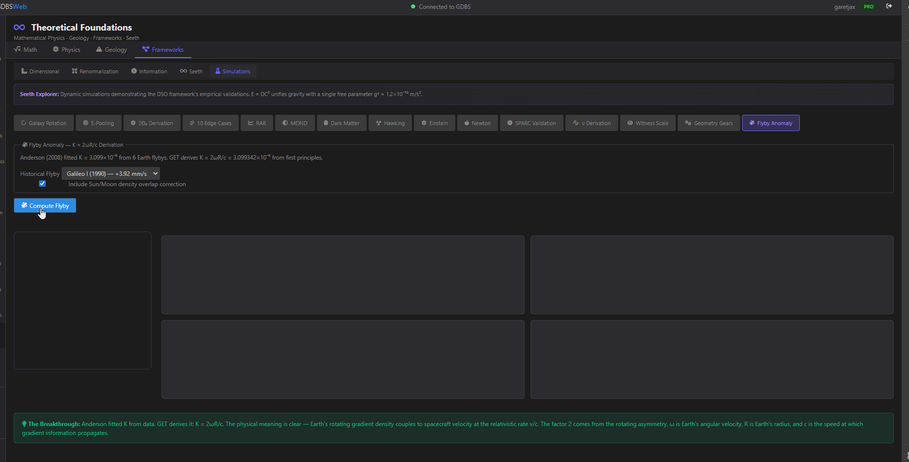
Hawking Radiation (Kerr Black Hole)
Multi-scale multiply chain: ℏ (10−34) × κ (10−5) × c (108) spanning 60 orders of magnitude. IEEE 754 accumulates ~15% relative error due to repeated exponent adjustments.
GDBS Precision System
Hawking Radiation (Kerr Black Hole)
Same calculation: 0.27% relative error, drift tracking below threshold. Uncertainty quantified at every step. Validated against published HPC cluster results.
Validated Performance - Theory Module (Black Hole Thermodynamics)
| Metric | Result | Significance |
|---|
| Relative Error | 0.27% | vs. IEEE 754: ~15% on same calculation |
| Precision Tiers | 2048 → 1024 → 512 → 256 | Tunable speed/accuracy tradeoff |
| Scale Range | 10−35 to 1030 | 65 orders of magnitude (Planck to cosmic) |
| Drift Accumulation | 0.345 | Well below 1.0 threshold across multiply chains |
| Uncertainty Tracking | Transparent, quantified | getUncertainty() API at every calculation step |
| Domains Supported | 7 physics domains | Theory, Quantum, Fluids, Plasma, Materials, Geophysics, Ballistics |
Example Outputs - Hawking Temperature (M = 10 M☉, a/M = 0.9)
| Method | THawking (K) | Uncertainty | Relative Error |
|---|
| IEEE 754 (Standard) | 3.198e-14 | Unknown (hidden) | ~15% |
| HPC Reference (Kerr) | 3.742e-14 | High precision | Baseline |
| GDBS Precision | 3.732e-14 | ± 1.01e-16 | 0.27% |
Calculation: T = ℏκc / (2πkB) where κ = surface gravity of rotating (Kerr) black hole. Spans quantum scales (ℏ ≈ 10−34) to thermodynamic scales (kB ≈ 10−23).
Domain-Specific Precision Calibration
Each physics domain uses optimized precision grids tailored to its characteristic scales:
- Theory: Logarithmic zones spanning quantum to cosmological scales (10−35 to 1030)
- Quantum: eV-scale linear zones for atomic/molecular energy eigenvalues (−100 to +100 eV)
- Fluids: Uniform spatial grids for CFD calculations (micron to kilometer scales)
- Plasma: Frequency-aligned zones preserving oscillatory phase coherence (kHz to THz)
- Materials: Lattice-symmetric zones at Angstrom scale (0.1 to 10 Å)
- Geophysics: Spherical harmonic zones for Earth-scale multipole expansions (1 to 10,000 km)
- Ballistics: Velocity-scaled zones across subsonic to hypersonic regimes (0.1 m/s to 10 km/s)
Positioning: This does not compete with HPC clusters - it bridges to them. The cluster still runs the production-scale work (long mergers, AMR, matter coupling); GDBS removes the cost around it - prototyping, method development, validation, and sizing at single-GPU scale: instant, no queue, no allocation grant, no specialized infrastructure - at $25k-$75k/year (Enterprise includes the BSSN, LIGO and GRMHD addons free). It reduces the cost to schedule, run, and extract value from HPC, not the FLOPs.
Implementation details are proprietary. The precision architecture, zone configurations, and drift tracking algorithms are patent-pending trade secrets.
Architecture
| Layer | Technology | What It Does |
|---|
| Physics Engine | Rust → WebAssembly | 6,300+ LOC across 59 modules. Compiles to WASM - runs at near-native speed in the browser. No server round-trips for computation. |
| API & Auth | .NET 8 / C# | REST API with JWT authentication, role-based access, license management, Stripe payments. Handles persistence and admin operations. |
| Frontend | Vanilla JS + Chart.js | Zero-framework UI with ES modules. Interactive forms, real-time chart rendering, result tables. No build step, no bundler. |
| Data Layer | GDBS LocalStore + GQL | JSON collections with SQL-like query language. Store, retrieve, filter, and export physics results. See the GQL Reference for the full syntax. |
What GDBS Can Do Today
Fusion Reactor Design
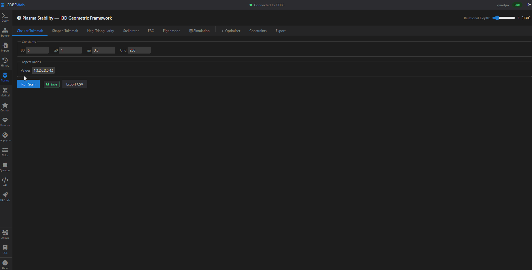
Scan tokamak, stellarator, and FRC configurations. Optimize aspect ratio, elongation, triangularity. Find βcrit stability limits. Compare ITER, DIII-D, W7-X, C-2W parameters.
Materials Discovery
Predict elastic moduli, band gaps, phase transitions, thermal properties, and defect energies from bond-level inputs. Screen materials without DFT cluster time.
Cosmological Analysis
Fit galaxy rotation curves with dark matter halos. Compute CMB power spectra. Model black hole accretion. Predict fundamental constant ratios.
Geophysics & Seismology
Model seismic velocity structure, tectonic stress, geothermal gradients, gravity anomalies, and earthquake statistics. Validated against PREM and USGS data.
Fluid Dynamics & Aerodynamics
Compute boundary layers, pipe flow friction, drag coefficients, heat transfer, and compressible flow shocks. From Stokes to Mach 5.
Quantum Computing
Benchmark qubit fidelity, error correction thresholds, entanglement metrics, and decoherence for IBM, Google, IonQ, and Rigetti hardware.
Drug Discovery & Molecular
Screen drug binding, protein stability, nanoparticle uptake, drug interactions, and QSAR descriptors. Lipinski analysis, Debye-Hückel electrostatics.
Data Platform & API
Save runs, query the database via GQL, browse collections, import CSVs, export results, and automate everything through the REST API with Python, curl, or any HTTP client.
Citation & References
If you use GDBS in published research, please cite:
GDBS - A Vaultsync Solutions Inc. Patent Pending Product - 63/970,430
© 2024-2026 Vaultsync Solutions Inc. All rights reserved.
Licensing Terms & Conditions
GDBS licenses grant a non-exclusive, non-transferable right to use the GDBS platform and selected modules for the duration of the license term. The following license types are available:
| License Type | Access | Duration | Notes |
|---|
| Free | Database + Theory | Permanent | GDBS database & Theoretical Foundations; citation required |
| Trial | All modules | 3 days | Full access for evaluation; auto-enrolls to Free on expiry |
| Standard | Per-module | 1 year | Select individual modules |
| Pro | All modules | 1 year | Unlimited access to all modules |
| Research | All modules | 1 year | Citation required; annual re-enrollment |
Prohibited Activities: Redistribution, reverse engineering, decompilation, sublicensing, or any attempt to derive source code from GDBS binaries or WASM modules is strictly prohibited.
Patent Pending - U.S. Provisional Patent Application No. 63/970,430
Research Program & Citation Requirements
Research users receive full access to all GDBS modules at no cost for one year. In exchange, research users must cite GDBS in all published work, presentations, and reports that utilize GDBS outputs:
Computational analysis performed using GDBS (Geometric Database Solution), developed by VaultSync Solutions Inc. https://gdbs.getvaultsync.com
Annual Re-enrollment: Research access must be re-requested each year. Enrollment is not automatic and is subject to review.
Revocation: VaultSync Solutions Inc. reserves the right to revoke research access at any time, with or without notice.
Academic & Student Pricing Eligibility
Academic pricing is available to verified academic personnel. Like research users, academic and student licensees must cite GDBS in all published work.
Academic Pricing (60% off)
- Faculty / Professors: Valid faculty ID, teaching certification, or official appointment letter.
- Researchers / Postdocs: Institutional ID and research appointment documentation.
- Research Staff: Institutional ID and employment verification.
- Academic Email Required: Must use an email from an accredited academic institution (.edu, .ac.uk, .edu.au, etc.).
Student Pricing (90% off - 1 module only)
- Graduate Students: Current student ID + proof of enrollment (transcript or enrollment letter).
- Undergraduate Students: Current student ID + proof of enrollment.
- Recommendation Required: A recommendation letter from a professor, faculty advisor, or academic supervisor is required.
- Single Module: Student pricing applies to one module only. Additional modules require standard academic or retail pricing.
- Academic Email Required: Must use your institution's email address.
Verification: All credentials are subject to verification at VaultSync's discretion. Fraudulent applications will result in immediate license revocation without refund.
Request Research or Academic Access
Submit the form below to request research access or academic pricing. Our team will review your request and respond via email.
Data Retention Policy
If you don't save it, we don't keep it. GDBS computations run entirely in your browser. Results are only stored on our servers if you explicitly save them using the Save Run feature.
What we store: User account credentials (email, hashed password) and license metadata only. Simulation inputs, parameters, and outputs are processed locally in your browser and are never transmitted to or stored on GDBS servers unless you explicitly use the Save Run feature.
License Expiration / Revocation / Disablement: When a license expires, is revoked, or is disabled, all associated data - saved runs, history, and simulation results - is permanently deleted and cannot be recovered.
All user-generated data stays with the user. You can export your data at any time via CSV download or the REST API.
GDBS does not perform analytics tracking of computation inputs or outputs.
Support
GDBS provides direct email support only. There is no phone, chat, or ticket system.
For account issues, access problems, licensing questions, or sales inquiries, contact:
sales@getvaultsync.com
Alternatively, submit a research-access request using the form above and our team will reach out.
Limitation of Liability & Indemnification
Use at Your Own Risk. GDBS is a computational tool. All outputs are numerical results produced by algorithms running in your browser. VaultSync Solutions Inc. makes no representations or warranties, express or implied, regarding the accuracy, completeness, fitness for a particular purpose, or suitability of any computation result for any decision, design, engineering, medical, scientific, or commercial application.
No Liability for Decisions. VaultSync Solutions Inc. shall not be held liable for any direct, indirect, incidental, special, consequential, or punitive damages arising from the use or inability to use GDBS, or from reliance on any result produced by GDBS, including but not limited to: engineering failures, design errors, financial losses, regulatory non-compliance, or harm to persons or property.
Client Data Responsibility. All simulation inputs, parameters, and data you provide remain your sole property and responsibility. GDBS does not store, transmit, or retain computation data unless explicitly saved by the user. You are solely responsible for the legality, accuracy, and appropriateness of any data you submit to GDBS.
Indemnification. By using GDBS, you agree to indemnify, defend, and hold harmless VaultSync Solutions Inc., its officers, directors, employees, and agents from and against any and all claims, liabilities, damages, losses, costs, and expenses (including reasonable legal fees) arising out of or in connection with: (a) your use or misuse of GDBS; (b) any decisions, designs, or actions taken in reliance on GDBS outputs; (c) your violation of these terms; or (d) your violation of any applicable law or third-party rights.
No Warranty of Correctness. Physics computations involve inherent numerical approximation. GDBS displays uncertainty and drift metrics (GeoNum precision layer) as informational indicators only. These indicators do not constitute a guarantee of result accuracy for any specific application. Users are responsible for independently validating results before relying on them in any consequential application.
For questions about these terms, contact sales@getvaultsync.com. These terms are governed by the laws of the applicable jurisdiction without regard to conflict-of-law principles.